Transform Coding and Compressive Sensing
It is now clear that we want to reduce the number of samples to represent some information. In this article, we'll talk about a method called transform coding which is used for the same purpose.
A signal \( \mathbf{f} \in \mathbb{R}^N \) can be represented in terms of \( N \times 1 \) basis vectors \( \left\lbrace \psi_i\right\rbrace _{i=1}^N\) as $$\mathbf{f} = \sum_{i=1}^{N}\; x_i\psi_i = \mathbf{\Psi x} $$.
A signal vector \( \mathbf{x} \in \mathbb{R}^{N \times 1} \) will be referred to as compressible if the magnitudes of its elements decay at a power law rate if sorted in decreasing order.
A signal \(\mathbf{f}\) is called \(K\)-sparse in \(\psi\) domain if only \(K\) out of \(N\) entries in coefficient vector \(\mathbf{x}\) are nonzero.
Transform Coding
Transform coding can be used to reduce number of samples to represent a signal if given signal is compressible or sparse. In transform coding, we first calculate coefficient vector \( \mathbf{x} \) using $$\mathbf{x} = \Psi^T\mathbf{f} $$Then we keep only \( K \) large entries and discard other \( N-K \) entries.
| Fig 1: Block diagram of transform coding |
Inefficiencies of Transform Coding
- The initial number of samples \(N\) maybe large even if \(K\) is small.
- All \(N\) coefficients have to be calculated even though \(N-K\) will be discarded.
- Locations of \(K\) coefficients have to be encoded which is an overhead.
At the receiver end, we have to decompress the signal. We use the assumption that coefficients for which locations are not encoded are zero.
Is there a way to bypass compression and decompression steps?
Yes. Compressive Sensing !
Compressive Sensing
The fundamental idea behind compressive sensing is that we want to acquire data in compressed form rather than first sampling the signal at a high rate and then compressing the sampled data.
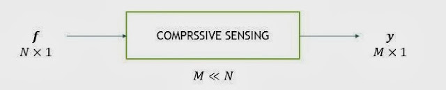 |
| Fig 2: Block diagram of compressive sensing |
This system can be represented as a matrix equation: $$ \mathbf{y} = \Theta \mathbf{f} $$ If \( \mathbf{f} \) is \(K\)-sparse in \(\Psi\) domain then above equation can be written as $$ \mathbf{y} = \Theta \Psi \mathbf{x} = \mathbf{Ax} $$ Where \( \mathbf{A} \) is \( M \times N \) matrix and \( M << N \).
If we observe above equation, we see that it represents an underdetermined system. So for a given \( \mathbf{y} \), there exist many \( \mathbf{x}\)'s which will satisfy this equation.
How do we solve this equation?
We've got a problem now. We acquired the data in compressed form. But we should be able to reconstruct the original signal with tolerable amount of error. We assumed earlier that signal is sparse in \( \Psi \) domain. We're gonna use this condition to solve the system. All we have to do is that find a unique \( K \)-sparse signal that satisfies this system.
How do we ensure all these conditions?
I said a lot about when we can reconstruct the signal from the acquired data. Seems like too many conditions, right? But good news, it all depends on measurement matrix, i.e. \( \mathbf{A} \). If \( \mathbf{A} \) satisfies two properties, there is high probability that original signal can be reconstructed exactly.
- Mutual Incoherence Property
- Restricted Isometry Property
Mutual Incoherence Property
Coherence between sensing matrix \( \Phi \) and representation matrix \( \Psi \) can be defined as $$ \mu( \Phi, \Psi ) = \sqrt{n}. \max_{k, j} |\left\langle \varphi_k, \psi_j\right\rangle | $$
Mutual incoherence property says that coherence between \( \Phi \) and \( \Psi \) should be as low as possible. It can be seen from theorem given below.
Fix \(\mathbf{f} \in \mathbb{R}^N\) and suppose that the coefficient equence \(\mathbf{x}\) of \(\mathbf{f}\) in the basis \(\Psi\) is \(K\) sparse. Select \(m\) measurements in the \(\Phi\) domain uniformly at random. Then if $$ m \geq C.\mu^2(\Phi, \Psi).K.\log N $$ for some positive constant \(C\), the signal can be reconstructed exactly with overwhelming probability.
It can easily be seen that less samples will be required if coherence is less.
Restricted Isometry Property
For each integer \(K = 1, 2, \dots\), define the isometry constant \(\delta_K\) of a matrix \(\mathbf{A}\) as the smallest number such that $$ \label{ripDef} (1 - \delta_K) ||\mathbf{x}||_{l_2}^2 \leq ||\mathbf{Ax}||_{l_2}^2 \leq (1 + \delta_K) ||\mathbf{x}||_{l_2}^2 $$ holds for all \(K\)-sparse vectors \(\mathbf{x}\). We will loosely say that a matrix \(\mathbf{A}\) obeys the RIP of order \(K\) if \(\delta_K\) is not too close to one.
The implication of above definition is that we don't want \(l_2\) norm of a signal to change much in dimensionality reduction process.
An equivalent description of the RIP is to say that all subsets of \(K\) columns taken from \(\mathbf{A}\) are nearly orthogonal. This is necessary to ensure the uniqueness of \(K\)-sparse solution.
There are many reconstruction algorithms available to reconstruct the signal with tolerable amount of error. I'll discuss them later.
I mostly referred to this paper for this blog post.